Chaos and Feigenbaum’s Constant#
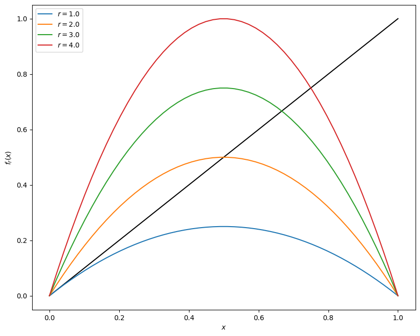
Here we consider the phenomena of period doubling in chaotic systems, which leads to universal behavior [Feigenbaum, 1978]. The quintessential system is that of the Logistic map:
which is a crude model for population growth. The interepretation is that \(r\) is proportional to the growth rate, and that \(x \in [0,1]\) is the total population as a fraction of the carrying capacity of the environment. For small \(x\), the population grows exponentially without bound \(x \mapsto r x\), while for large \(x \approx 1\) the population rapidly declines as the food is quickly exhausted and individuals starve.
def f(x, r, d=0):
"""Logistic growth function (or derivative)"""
if d == 0:
return r*x*(1-x)
elif d == 1:
return r*(1-2*x)
elif d == 2:
return -2*r
else:
return 0
The behaviour of this system is often demonstrated with a cobweb plot:
from matplotlib.animation import FuncAnimation
from IPython.display import HTML
class CobWeb:
"""Class to draw and animate cobweb diragrams.
Parameters
----------
x0 : float
Initial population `0 <= x0 <= 1`
N0, N : int
Skip the first `N0` iterations then plot `N` iterations.
"""
def __init__(self, x0=0.2, N0=0, N=1000):
self.x0 = x0
self.N0 = N0
self.N = N
self.fig, self.ax = plt.subplots()
self.artists = None
def init(self):
return self.cobweb(r=1.0)
def cobweb(self, r):
"""Draw a cobweb diagram.
Arguments
---------
r : float
Growth factor 0 <= r <= 4.
Returns
-------
artists : list
List of updated artists.
"""
# Generate population
x0 = self.x0
xs = [x0]
for n in range(self.N0 + self.N+1):
x0 = f(x0, r=r)
xs.append(x0)
xs = xs[self.N0:] # Skip N0 initial steps
# Manipulate data for plotting
Xs = np.empty((len(xs), 2))
Ys = np.zeros((len(xs), 2))
Xs[:, 0] = xs
Xs[:, 1] = xs
Ys[1:, 0] = xs[1:]
Ys[:-1, 1] = xs[1:]
Xs = Xs.ravel()[:-2]
Ys = Ys.ravel()[:-2]
if self.N0 > 0:
Xs = Xs[1:]
Ys = Ys[1:]
x = np.linspace(0,1,200)
y = f(x, r)
title = f"$r={r:.2f}$"
if self.artists is None:
artists = self.artists = []
artists.extend(self.ax.plot(Xs, Ys, 'r', lw=0.5))
artists.extend(self.ax.plot(x, y, 'C0'))
artists.extend(self.ax.plot(x, x, 'k'))
self.ax.set(xlim=(0, 1), ylim=(0, 1), title=title)
artists.append(self.ax.title)
else:
artists = self.artists[:2] + self.artists[-1:]
artists[0].set_data(Xs, Ys)
artists[1].set_data(x, y)
artists[2].set_text(title)
return artists
def animate(self,
rs=None,
interval_ms=20):
if rs is None:
# Slow down as we get close to 4.
x = np.sin(np.linspace(0.0, 1.0, 100)*np.pi/2)
rs = 1.0 + 3.0*x
animation = FuncAnimation(
self.fig,
self.cobweb,
frames=rs,
interval=interval_ms,
init_func=self.init,
blit=True)
display(HTML(animation.to_jshtml()))
plt.close('all')
cobweb = CobWeb()
cobweb.animate()
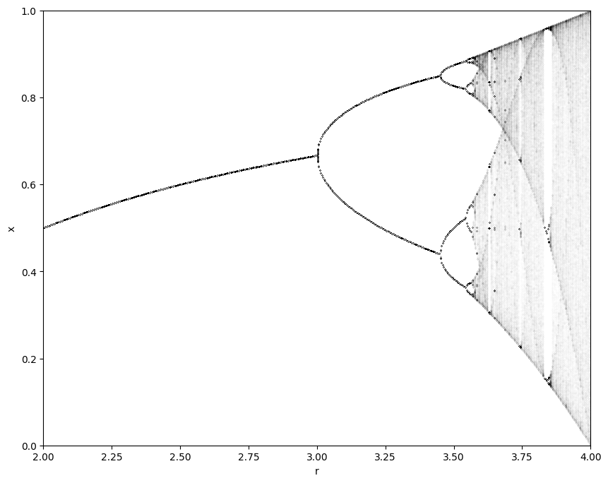
Notice that as the growth constant increases, the population first stabilizes on a single fixed-point, but then this expands into a cycle of period 2, then a cycle of period 4 etc. This is called period doubling, and this behaviour can be summarized in a bifircation diagram.
Bifurcation Diagrams#
Here we develop an algorithm for drawing a high-quality bification diagram. We start with a simple algorithm that simply accumulates \(N\) iterations starting with \(x_0 = 0.2\) at a set of \(N_r\) points between \(r_0=2.0\) and \(r_1=4.0\).
fig, ax = plt.subplots()
r0 = 2.0
r1 = 4
Nr = 500
N = 200
x0 = 0.2
rs = np.linspace(r0,r1,Nr)
for r in rs:
x = x0
xs = []
for n in range(N):
x = f(x, r=r)
xs.append(x)
ax.plot([r]*len(xs), xs, '.', ms=0.1, c='k')
ax.set(xlabel='$r$', ylabel='$x$');
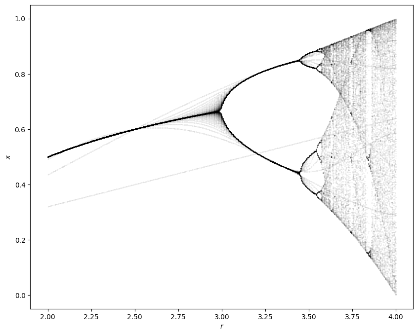
This works reasonably well, but has several artifacts. First, note the various curves - these are reminants of the choice of the initial point. Instead, we should iterate through some \(N_0\) iterations to allow the system to stabilize, then start accumulating.
fig, ax = plt.subplots()
N0 = 100
rs = np.linspace(r0,r1,Nr)
for r in rs:
x = x0
for n in range(N0):
x = f(x, r=r)
xs = []
for n in range(N):
x = f(x, r=r)
xs.append(x)
ax.plot([r]*len(xs), xs, '.', ms=0.1, c='k')
ax.set(xlabel='$r$', ylabel='$x$');
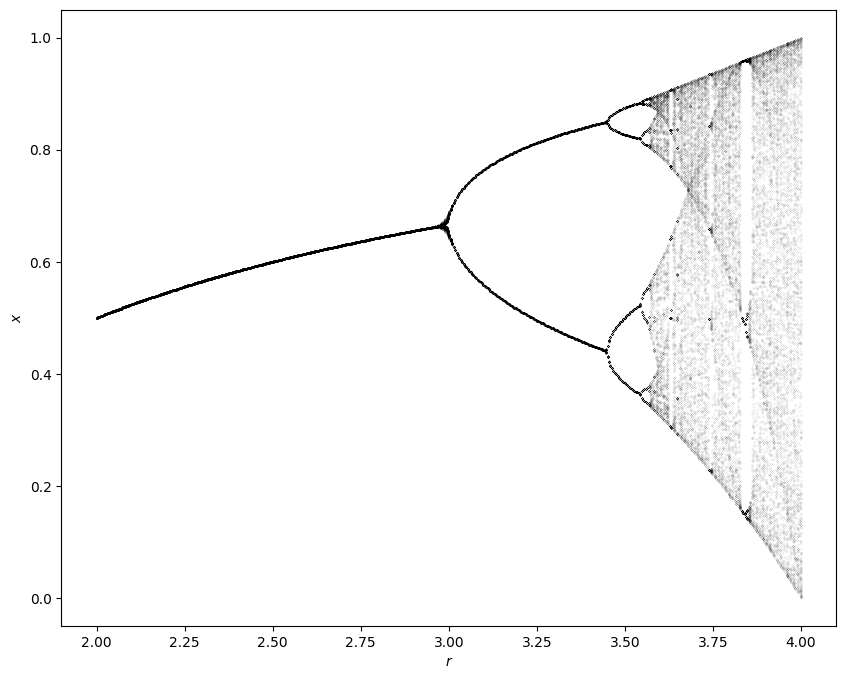
This is better, but the bifurcation points are still blurry because it takes a long time for the system to settle down there. One solution is to increase \(N_0\), but this will increase the computational cost. Another is to use the last iteration \(x\) from the previous \(x\) as \(x_0\) which should put us close to the final attractor. This latter solution works well without increasing the computational cost:
fig, ax = plt.subplots()
N0 = 100
x = x0
rs = np.linspace(r0,r1,Nr)
for r in rs:
# x = x0 # Use the previous value of x
for n in range(N0):
x = f(x, r=r)
xs = []
for n in range(N):
x = f(x, r=r)
xs.append(x)
ax.plot([r]*len(xs), xs, '.', ms=0.1, c='k')
ax.set(xlabel='$r$', ylabel='$x$');
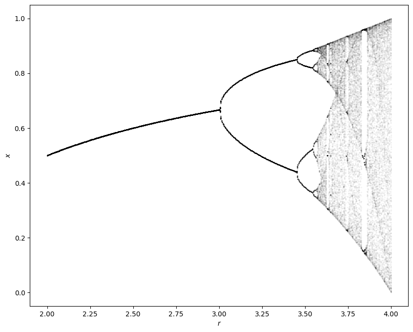
There are further refinements one could make: for example, when the system converges quickly to a low period cycle, we still perform \(N\) iterations and plot \(N\) points. One could implement a system that checks to see if the system has converged, then finds the period of the cycle so that only these points are plotted. Such a system should fall back to the previous method only when the period becomes too large. Another sophisticated approach would be to track the curves on the bifurcation plot and plot these as smooth curves. These require some book keeping and we keep our current algorithm which we now code as a function. A final modification we add is allowing the points to be transparent which enables us to see the relative density of points.
def bifurcation(r0=2, r1=4, Nr=500, x0=0.2, N0=500, N=2000, alpha=0.1,
rs_xs=None):
"""Draw a bifurcation diagram"""
if rs_xs is not None:
rs, xs = rs_xs
else:
rs = np.linspace(r0,r1,Nr)
xs = []
x = x0
for r in rs:
for n in range(N0):
x = f(x, r=r)
_xs = [x]
for n in range(N):
_xs.append(f(_xs[-1], r=r))
xs.append(_xs)
_rs = []
_xs = []
for r, x in zip(rs, xs):
_rs.append([r]*len(x))
_xs.append(x)
plt.plot(_rs, _xs, '.', ms=0.1, c='k', alpha=alpha)
plt.axis([r0, r1, 0, 1])
plt.xlabel('r')
plt.ylabel('x')
return rs, xs
rs_xs = bifurcation()
Fixed Points#
The fixed points can be easily deduced by finding the roots of \( x = f^{(n)}(x)\) where the power here means iteration \(f^{(2)}(x) = f(f(x))\)
Period 1#
Here are the period 1 fixed points. The solution at \(x=0\) is trivial, but there is a nontrivial solution \(x = 1 - r^{-1}\) if \(r\geq 1\):
---------------------------------------------------------------------------
TypeError Traceback (most recent call last)
Cell In[11], line 2
1 xs = np.linspace(0, 1.0, 100)[1:-1]
----> 2 plt.plot(r1(xs), xs, 'r')
3 bifurcation(rs_xs=rs_xs);
TypeError: 'int' object is not callable
Period 2#
For period 2 we have the solutions for the period 1 equations since these also have period 2, and two new solutions of which only one is positive:
---------------------------------------------------------------------------
TypeError Traceback (most recent call last)
Cell In[13], line 2
1 xs = np.linspace(0, 1.0, 100)[1:-1]
----> 2 plt.plot(r1(xs), xs, 'r')
3 plt.plot(r2(xs), xs, 'g')
4 bifurcation(rs_xs=rs_xs);
TypeError: 'int' object is not callable
Period 3 Implies Chaos#
In 1975, Li and Yorke proved that Period 3 Implies Chaos in 1D systems by showing that if there exists cycles with period 3, then there are cycles of all orders. Here we demonstrate the period 3 solution.
---------------------------------------------------------------------------
NameError Traceback (most recent call last)
Cell In[14], line 1
----> 1 res = sympy.factor((fn(3) - x)/x/(r-r1s[0])/(x-1))
3 coeffs = sympy.lambdify([r], sympy.Poly(res, x).coeffs(), 'numpy')
5 def get_x3(r, _coeffs=coeffs):
NameError: name 'sympy' is not defined
Exact solution for \(r=4\): Angle doubling on the unit circle#
The chaos at \(r=4\): \(x\mapsto 4x(1-x)\) is special in that the evolution admits an exact solution. Start with the identity:
This suggests letting \(x_n = \sin^2\theta_n\) and \(x_{n+1} = \sin^2\theta_{n+1}\) which now yields the trivial map \(\theta \mapsto 2\theta\) which has the explicit solution \(\theta_n = 2^n\theta_0\). Hence the logistic map with \(r=4\) has the solution:
This evolution is equivalent to moving arround a unit circle by doubling the angle at each step. If \(\theta_0\) is a rational fraction of \(2\pi\) then the motion will ultimately become periodic, but if \(\theta_0\) is an irrational factor of \(2\pi\), then the motion will never be periodic.
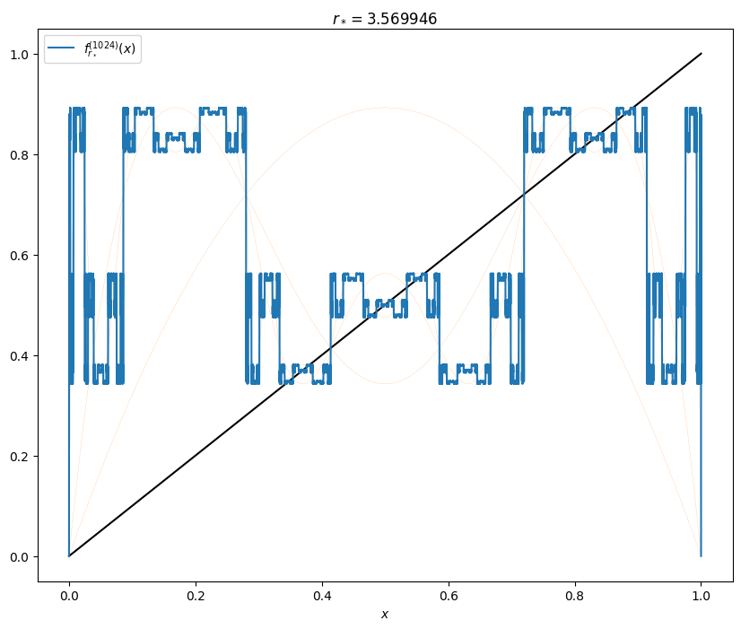
Feigenbaum Constants#
First we define some notation. Let \(r_{n}\) be the smallest value of the growth parameter where the period bifurcates from \(2^{n-1}\) to \(2^{n}\). Define the iterated function as:
The first bifurcation point is at \(r_{1} = 3\), \(x_{1} = 2/3\), i.e. the solution to \(x_1 = f_{r_1}(x_1)\). At this point, the fixed point becomes unstable: \(\abs{f'_{r_{1}}(x_{1})} = 1\). Now, since \(x_{1}\) is a fixed point of \(f_{r_1}(x)\), it must also be a fixed point of \(f^{(2)}_{r_1}(x)\). We plot both of these below, as well as \(f^{(2)}_{r_1+\epsilon}(x)\) for a slightly larger \(r = r_1 + \epsilon\):
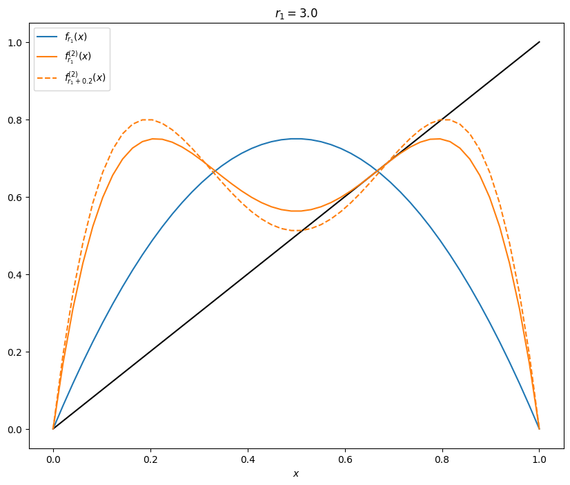
Notice the behaviour that, at this shared fixed point, \(f^{(2)}_{r_1}{}'(x) = \bigl(f'_{r_1}(x)\bigr)^2 = 1\). As we increase \(r = r_1+\epsilon\), this steepens and the two new fixed points move outward.
We now look at \(f^{(2)}_{r_2}(x)\) and \(f^{(4)}_{r_2}(x)\), where we see the same behaviour about both of the new fixed points:
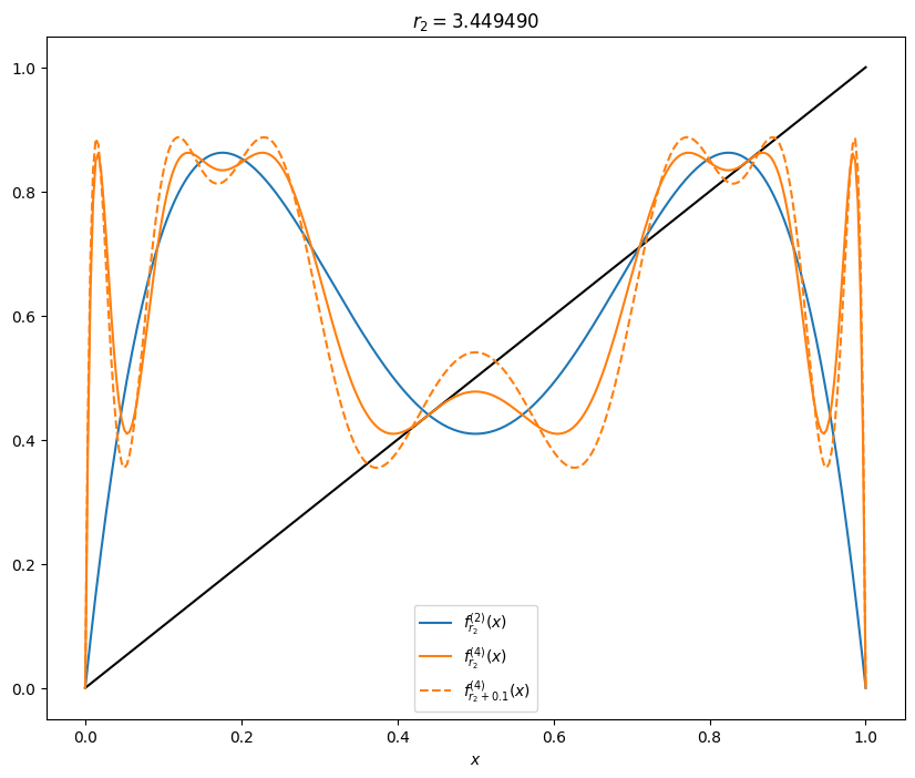
(see Weisstein, Eric W. “Logistic Map”).
\(n\) |
\(r_n\) |
\(\delta_n = \frac{r_{n}-r{n-1}}{r_{n+1}-r{n}}\) |
|---|---|---|
0 |
1 |
|
1 |
3 |
|
2 |
3.449490 |
|
3 |
3.544090 |
|
4 |
3.564407 |
|
5 |
3.568750 |
|
6 |
3.56969 |
rn = np.array([1.0, 3.0, 1+np.sqrt(6),
3.5440903595519228536, 3.5644072660954325977735575865289824,
3.568750, 3.56969, 3.56989, 3.569934, 3.569943, 3.5699451,
3.569945557
3.5699456718709449018420051513864989367638369115148323781079755299213628875001367775263210342163
])
Mitchell Feigenbaum [Feigenbaum, 1978] poin